Data manipulation is a foundational skill of any good scientist. The ability to filter, select, mutate, and transform is essential. While you may be introduced to these skills early on, mastering them is a long journey.
1 Introduction
Welcome to “The Basics of Data”, after some gentle nudging I’m going to take a gigantic step back in terms of what I’ve been blogging about and really focus on the absolute basics. In this session we are going to explore how you would start getting into data analysis within your Integrated Developer Environment (AKA, your IDE, AKA Positron or RStudio). Specifically we will explore some basic coding actions that you will encounter when working with scientific data, this includes:
loading a dataset,
filtering,
selecting,
grouping,
mutating,
and summarising.
To compliment this we will also touch on some important R concepts and coding “best practices” as we work through the points above.
2 Loading Data
The first thing we are going to do is load in some data that we can practice on. This data is not from your local machine, this data is shipped within a specific R package (palmerpenguins). When you install an R package, you usually also install some practice data. Actually, from the moment you download R you also download additional practice datasets. These datasets are shipped with R for this exact purpose - testing and learning.
Code
#install the palmerpenguins package#install.packages("palmerpenguins")#to load in data that comes with R, we can just call the data like it is a variableour_data <- penguins#if you want to see all of the data that comes with R you can run the following code:#data()
3 Exploring Data
There are lots of ways to visually/manually explore the data. If this was data you had on your local machine you could of course open it in excel and take a look around, however in this case it isn’t. Additionally, you may one day work with data that is too large to open in excel. So how else can we look at the data? There are two main coding methods. The first is head():
Code
#you can use head() to view a subset of the data. It prints the data almost exactly as it looks in the dataframehead(our_data)
  species    island bill_len bill_dep flipper_len body_mass    sex year
1  Adelie Torgersen     39.1     18.7         181      3750   male 2007
2  Adelie Torgersen     39.5     17.4         186      3800 female 2007
3  Adelie Torgersen     40.3     18.0         195      3250 female 2007
4  Adelie Torgersen       NA       NA          NA        NA   <NA> 2007
5  Adelie Torgersen     36.7     19.3         193      3450 female 2007
6  Adelie Torgersen     39.3     20.6         190      3650   male 2007
Code
#head() defaults to the first 6 rows of data, but you can define a specific number as the second argument#head(our_data, 10)
The second is str():
Code
#the second option is to use the str() function (short for "structure")str(our_data)
'data.frame':   344 obs. of  8 variables:
 $ species    : Factor w/ 3 levels "Adelie","Chinstrap",..: 1 1 1 1 1 1 1 1 1 1 ...
 $ island     : Factor w/ 3 levels "Biscoe","Dream",..: 3 3 3 3 3 3 3 3 3 3 ...
 $ bill_len   : num  39.1 39.5 40.3 NA 36.7 39.3 38.9 39.2 34.1 42 ...
 $ bill_dep   : num  18.7 17.4 18 NA 19.3 20.6 17.8 19.6 18.1 20.2 ...
 $ flipper_len: int  181 186 195 NA 193 190 181 195 193 190 ...
 $ body_mass  : int  3750 3800 3250 NA 3450 3650 3625 4675 3475 4250 ...
 $ sex        : Factor w/ 2 levels "female","male": 2 1 1 NA 1 2 1 2 NA NA ...
 $ year       : int  2007 2007 2007 2007 2007 2007 2007 2007 2007 2007 ...
Code
#this option show the data in a slightly different way and tells us about column type (factor, number, int, str)
However by far the easiest way to view and explore the data is using the built in data explorer. Simply click on the table icon next to your data in the variable pane off to the right of the IDE, or if you wanted to code it, use View() (with a capital v).
Code
View(our_data)
With the data explorer you can learn pretty much anything you want. It is also interactive; you can filter, sort, inspect, etc.
Note
The data explorer is emphermeral - the changes you make to the dataset are not permanent and do not make changes to the actual data that you have loaded in.
3.1 Loading Your Own Data
We will take a quick detour here to discuss loading your own local data, this is important because loading data local data is actually one of the biggest frustrations of a budding data analyst. The crux of the issue is that if you wanted to load data from your local machine you would need to make sure the computer knows where to look, and importantly, you need to understand how pedantic computers are about finding things:
If the file you want to load is at: “C:_file.csv”
and you tell the computer you want: “C:_file.csv”
It will fail (captial M).
If the file you want to load is at: “C:_folder_file.csv”
and you tell the computer you want: “C:_file.csv”
It will fail (its not looking in the sub folder).
If the file you want to load is at: “C:_folder_file.csv”
and you tell the computer you want: “C:_folder_file.xlsx”
It will fail (wrong extension).
If you use the wrong load function it will fail
If you use the wrong function arguments it will fail
If you use the wrong code syntax it will fail
If you don’t assign the output to an object it will (kind of) fail
This is not intended to scare you, but rather to acknowledge how annoying computers can be, and reassure you that everyone feels this pain to begin with. So, when you load your own data pay very close attention to each of the above possibilites. You should also make heavy use of Positron “project” folders, and R “Rproject” files (google them).
4 Understanding Data Types
After looking at the data you have probably already noted there are data types such as factor, string, int, num, etc. If you decide to go down the road of being a “coder” you will need to understand the distinctions between these very very well. However, at this stage simply being aware of data types and their basic interactions is probably enough.
As you might expect, certain data types don’t work well together. For instance, you can’t sum a string (text) and an integer (number) together - how would that even work?
Code
#create a string and int objectmy_str <-"this is a string"my_int <-123#try to add the two variables togethermy_str + my_int
Error in my_str + my_int: non-numeric argument to binary operator
This is just about the only super critical aspect to be aware of and can be the cause of a lot of annoying errors. This is because you can enter a number (integer) as a string if you put the number in quotes:
Code
#create a string and int objectmy_str <-"123"my_int <-123#try to add the two variables togethermy_str + my_int
Error in my_str + my_int: non-numeric argument to binary operator
The important thing to realise here is that a dataframe might have a column full of numbers, but it is encoded as a string. If you don’t look closely it can catch you off guard.
5 Creating Variables
This is also a good point to touch on creating objects and assigning. The format is as follows:
object(name) <- information(data)
Without assigning data to an object, the data is just printed to the console and is not “saved” in your environment. I.e. it would not be in the variable pane on the right of your IDE. Assigning data to an object that already exists overwrites the existing data within the object, be careful not to delete previous work this way. (You can add things to existing objects, but we will not cover that today).
Make sure to name objects well as it will save you a lot of time and confusion in the future. Naming objects follows a similar logic to what we have discussed before, the rules for naming objects are:
An object name must start with a letter and can be a combination of letters, digits, period(.) and underscore(_). If it starts with period(.), it cannot be followed by a digit.
An object name cannot start with a number or underscore (_)
Object names are case-sensitive (age, Age and AGE are three different objects)
Reserved words cannot be used as objects (TRUE, FALSE, NULL, if…)
Error in parse(text = input): <text>:2:2: unexpected symbol
1: #no
2: _my_object
    ^
6 Manipulating Data
Data manipulation is the most common thing you will be required to do as a ecologist/scientist/consultant/etc. The basic workflow would be to:
Get some data in (either you collected it yourself or someone else did)
Analyse the data
Draw conclusions
Write a report
Data manipulation is the first step in analysing the data, it means organisating your data, preparing your data, cleaning your data, and selecting necessary aspects of your data. Once you have done this, you can then analyse.
You can do all of these tasks in base R, but there are packages that have been specifically designed to improve R’s capacity/speed/legibility. We are going to use both tidyr and dplyr, these are both part of the “tidyverse” set of packages.
Code
library(tidyr)library(dplyr)
Together these packages allows us to do pretty much all the tasks we could ever possibly want.
6.1 Filtering Data
To filter data we use the filter() function (duh). But we need to be clear that filter works on rows, that is to say that you define a condition, and the filter checks if that condition is met per row. An example will clarify this:
Code
#filter our dataset for only 1 species of penguinchinstrap_penguins <-filter(our_data, species =="Chinstrap")
As you can see we are only keeping rows that have the species “Chinstrap”.
Note
Use the data viewer to inspect this new dataset.
Caution
A common mistake is to use = (equals) when you mean == (is equal). The single equals sign = means “this is now”, the double equals sign == means “this is the same as”. It is a very subtle difference with big consequences. For example:
Code
#assign using single equalsmy_object ="Chinstrap"
What this does is create an object called species with the contents of “Chinstrap”, it is saying that my_object is now “Chinstrap”. However, in the filter() function what we want to ask is which rows contain “Chinstrap” or which rows are equal to “Chinstrap” already. For example:
Code
#overwrite the previous object, its content is now "Adelie"my_object ="Adelie"#compare our object to the text "Chinstrap", are they the same? (TRUE or FALSE)my_object =="Chinstrap"
[1] FALSE
Using a single equals creates/overwrites an object. Using a double equals is a comparison between two objects:
Code
#compare our object to the text "Adelie", are they the same? (TRUE or FALSE)my_object =="Adelie"
[1] TRUE
Therefore, you can see that when you are filtering what you want to do is ask for rows where species is the same as “Chinstrap”, but if you use only one equals, what you are actually doing is saying the entire species column should now have the contents of “Chinstrap”.
There are a range of other operators (=, ==, <-, +, -, %%, <, >, !=, etc.) However, the = and == operators are essential not to get confused.
6.2 Select Data
Conversely to filter, the select() function works on columns. As you might expect, you use the select() function to select the columns that you want:
Code
#use select on our data to only keep the species and bill length columnsspecies_bill_length <-select(our_data, c(species, bill_len))
Selecting columns is very simple to understand, but there are a few tricks to learn, some of the easiest are:
You can reverse your selection using an exclamation mark or minus symbol: select(our_data, !c(species, bill_len))
You can select by column index: select(our_data, 1:3)
You can use helper functions to perform complex selections: select(our_data, starts_with("prefix_"))
Caution
the c() inside the select() function stands for concatenate, it means to group up together. When we want a bunch of things to be recognised as one thing we use the c() function. This happens very often and will become second nature. Forgetting to use c() is a very common beginner mistake as it is not immediately intuitive to use it.
6.3 Selecting AND Filtering
Together the filter() and select() functions allow us to cut our data down to only the rows and columns we are interested in. They form quite a powerful pair, and have an impressive amount of flexibility built in to allow for all kinds of shenanigans. We can demonstrate this below.
This is also a good time to introduce the “pipe” which looks like this |> or like this %>%. |> is the base R version of the pipe, in almost every instance I would reccomend using this version as it will do everything you need without having to install another package. %>% is from the magrittr package, it is the original pipe and existed long before |> did, you will see the %>% version in older code. It is technically more powerful, but the use cases where this matters are extremely limited.
The pipe is used to chain functions like filter() and select() together. In a basic sense, what the pipe does is replace the first argument in the function to its right with the object to the left of the pipe. For example, x |> f(1) is the same as f(x, 1). There are more complex ways to use the pipe, but they are not relevant right now.
The shortcut to enter a pipe is “ctrl” + “shift” + “m”.
Lets see the pipe in action:
Code
#here is the old methodchinstrap_penguins <-filter(our_data, species =="Chinstrap")cleaned_data_old_method <-select(chinstrap_penguins, c(species, bill_len))#and here is now it is done using the new methodcleaned_data_new_method <- our_data |>filter(species =="Chinstrap") |>select(c(species, bill_len))
We can see that for starters, less code needs to be written, but also less objects are created and the goal of the code is easier to understand. We can clearly see that the filter() and select() functions are meant to be working together to achieve something.
Lets write a slightly more complicated example:
Code
#write a more complicated workflow to demonstrate the benefit of pipinga_complex_output <- our_data |>filter(species =="Chinstrap"| species =="Adelie") |>#the | symbol means "or"select(!flipper_len) |>filter(island =="Biscoe") |>select(c(species, bill_len)) |>filter(bill_len <37.8)
A few things to note;
it is best practice to start a new line after a pipe - particularly for long pipes
this particular code is just for demonstration purposes, yes you can write this more efficently
I introduced the | operator, this means “or”. The filter will keep rows that meet either of the conditions
6.4 Mutating Data
After filtering and selecting the data we want, the next thing we often want to do is perform some kind of transformation (AKA mutation) of the data. This is achieved using the mutate function. The mutate function is the ultimate workhorse, the amount of things you can do with it is insane, below are just some very basic examples:
Code
#create a new columnour_mutated_data_1 <- our_data |>mutate(MyNewColumn ="Hello")#update an existing columnour_mutated_data_2 <- our_data |>mutate(Species ="overwritten")#calculate something based on other columns you can use operators like +, -, >, <, ==our_mutated_data_3 <- our_data |>mutate(LenAndDep = bill_len < bill_dep)
And just to demonstrate, here is a more complicated example (you don’t need to follow this right now):
Code
#here is a more complicated example of a mutate - they can get even MORE complicateda_more_complex_mutate <- our_data |>mutate(ExampleColumn =case_when( species =="Chinstrap"~"I love this guy", species =="Adelie"~"Nah these guys suck", T ~"Meh, their ok" ))
Note
Open the data explorer and see if you can follow the logic of the mutate.
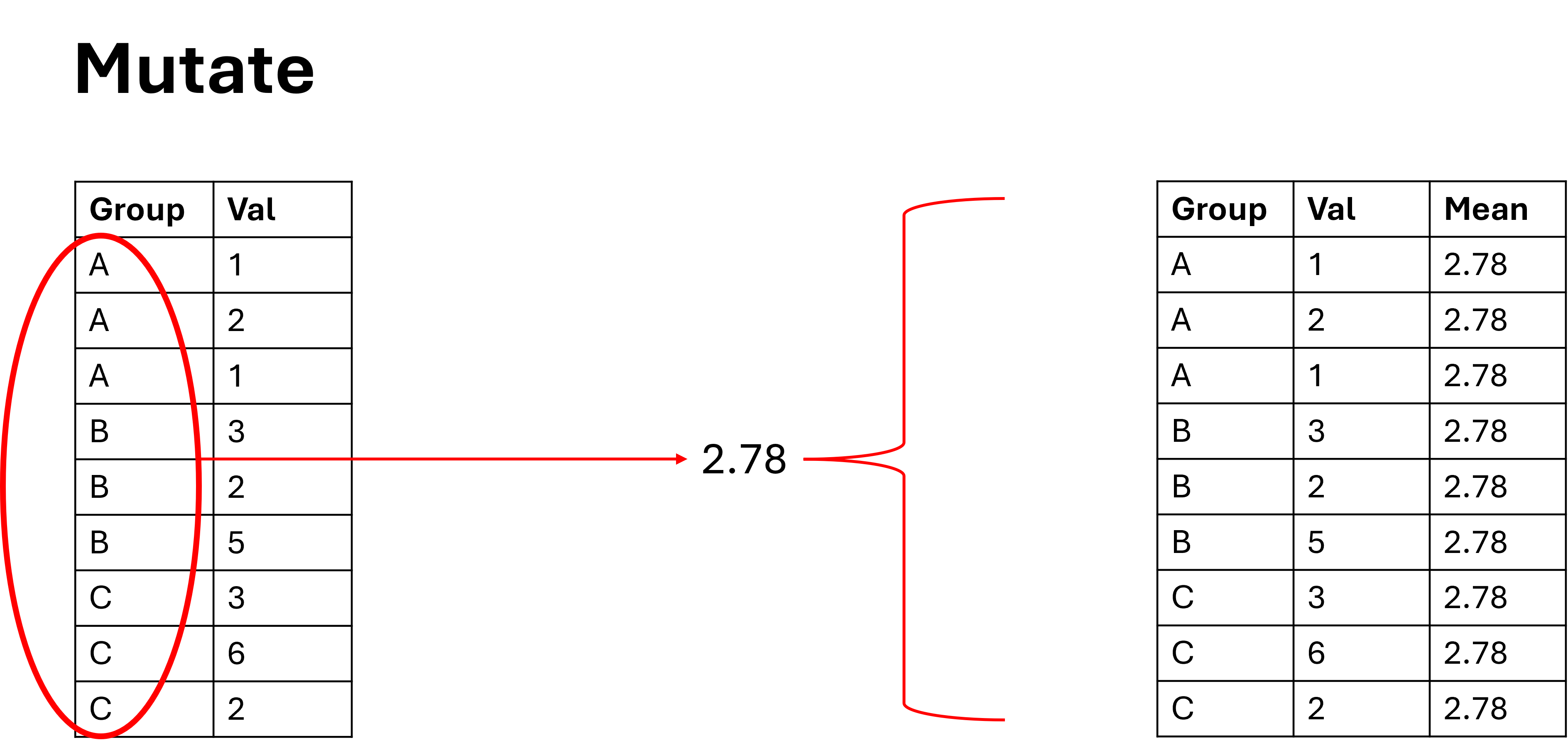
However, the mutate function on its own is still limited. This is because mutate() is applied per row. That is, if you have a dataframe with 10 rows and you write a mutate function, it will return a column with 10 rows. But… what if you want to calculate the mean value of all 10 rows? or what if you have two groups within the 10 rows, and you want to calculate a mean for each group?… And this problem is not just restricted to mutate(), you may also come across this issue when using the filter function among others.
We can visualise this as follows:
An Example of an Ungrouped Mutate
6.5 Group By
This is where the function group_by() comes in. We use group_by() to define groups in the dataframe to apply operations to. The group_by function doesn’t do anything on its own, and needs to be used in conjuction with other functions to have any affect. Below is an example of a grouped and ungrouped data transformation:
when you group data, never forget to ungroup the data at the end of the function. Think of the group_by() function as tag that is applied to the dataset, that tag will stick to the dataset forever, and will apply to all future functions unless you ungroup the data afterwards.
I introduce the mean() function, it does as you expect and returns the mean of the numbers it was provided. Because we grouped data by species, it will provide the mean bill length for each species.
the “na.rm” argument means remove NA values from the mean calculation
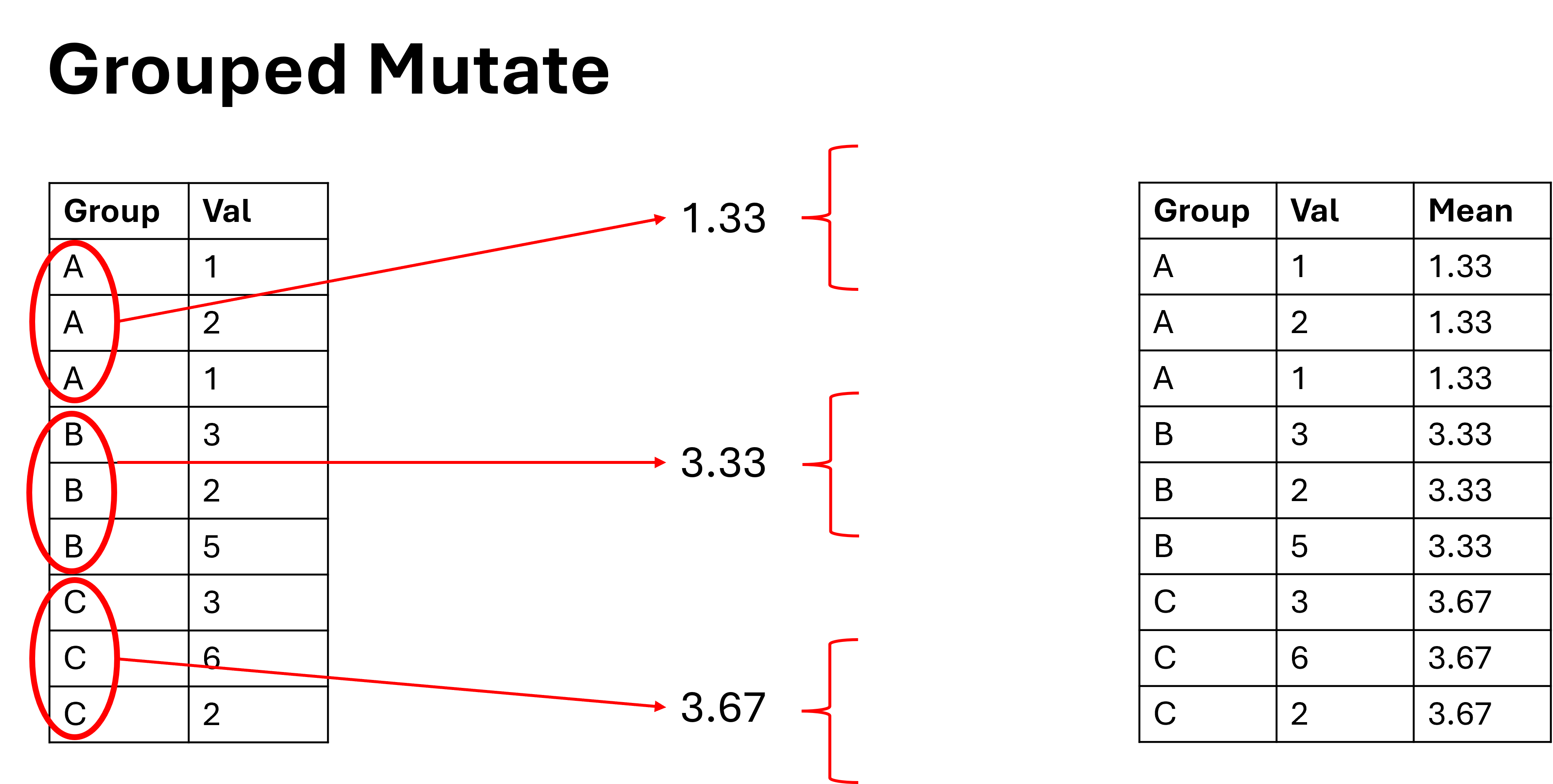
The grouping function allows us to perform operations on distinct groups in the data without having to physically split the dataset up into lots of different tables. However as you may have noticed, when we grouped and mutated the dataframe didn’t actually get any smaller (i.e. decrease in rows). This is a common confusion among beginner coders, you grouped the data up, why is it still the same size? Because decreasing rows can sometimes remove data that you were still interested in.
We can visualise this as follows:
An Example of a Grouped Mutate
Let’s imagine that you have a two step process:
Calculate the mean of some group
Calculate the deviation of each value from the mean
Because the dataframe didnt get any smaller, this is actually very easy and we can continue to do rowwise operations.
If the data frame got smaller, this would be very hard indeed. However, sometimes we do want to reduce the dataframe.
6.6 Summarise
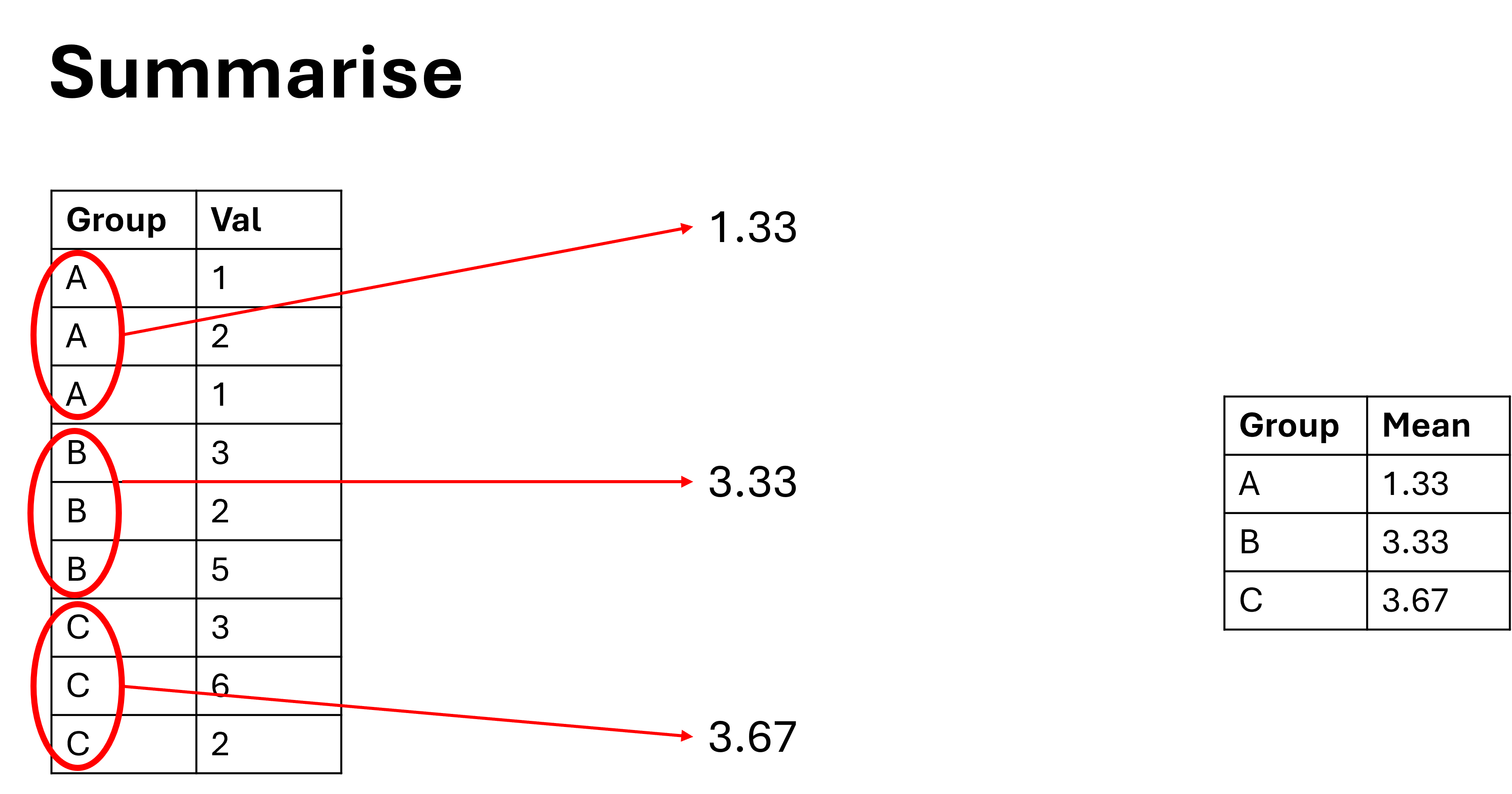
Enter summarise(), the final function we will look at today. This function is very similar to mutate(), but its interaction with the group_by() function is slightly different. Where mutate will return the same number of rows as was entered, summarise will reduce the number of rows down to the bare minimum. Again, this is best seen with an example:
The code is written in almost the same way, but the outputs are very different. Further, an important thing to realise with summarise, is it will naturally select only the relevant rows. For example, if you group by species, and summarise bill length, then it will only keep the species and bill length columns. This can catch beginners offguard as they wonder where their data went:
Code
#demonstrate the selection properties of the summarise functionour_summarised_data_2 <- our_data |>group_by(species) |>summarise(avg_bill_len =mean(bill_len, na.rm = T))
We can visualise this as follows:
An Example of Summarising
7 Final Thoughts
Coding is a long journey, and you will learn as you go. However, there are some good habits to get into right from the start that will help you read, write, and understand your own code when you come back to it. These include:
Naming variables well
Documenting your code (writing comments or explanations), this also helps you learn
Putting spaces between chunks of code, this help separate ideas
Starting a new line if the current line is too long
And thats about it! See you next time.
Thanks For Reading!
If you like the content, please consider donating to let me know. Also please stick around and have a read of several of my other posts. You'll find work on everything from simple data management and organisation skills, all the way to writing custom functions, tackling complex environmental problems, and my journey when learning new environmental data analyst skills.