Going Loopy for For Loops

1 Introduction

Here’s the scene, you’ve started on your R coding journey, know how to create an object, how to discern between vectors and lists, maybe even written a few short scripts. Then all of a sudden your professor/teacher/boss pulls a fast one on you and introduces for loops. For loops? What are they? How’s that work? Whats going on? You struggle through and complete the task, but didn’t quite understand what was going on when they explained it to you… Well at least that’s how it went for me.

In this post I wanted to quickly talk about for loops in R, specifically, I’m looking to cover:

• What is really happening in a for loop
• Where you can go to read about for loops in much (much) more detail
• Why you might want to write a for loop
• How you can start to write your own loops
• And ironically, why I actually try to avoid using for loops

2 For Loops

Realistically, all a for loop does, is say “do this bit of code again and again until I say stop”. Lets imagine a completely unrealistic scenario where your boss asks you to write out the numbers 1 to 10. Why are they asking you to do this? I don’t know, that’s not really the point. So you do it:

#manually write out a list of numbers from 1 to 10
my_list_numbers <- c(1,2,3,4,5,6)

#print these numbers
print(my_list_numbers)

[1] 1 2 3 4 5 6

Okay, clearly this is a dumb way to do this, I’m not even going to write out the whole thing. Instead, lets create our first for loop:

#write a for loop to print the numbers 1 to 10
for (i in 1:10){print(i)}

[1] 1
[1] 2
[1] 3
[1] 4
[1] 5
[1] 6
[1] 7
[1] 8
[1] 9
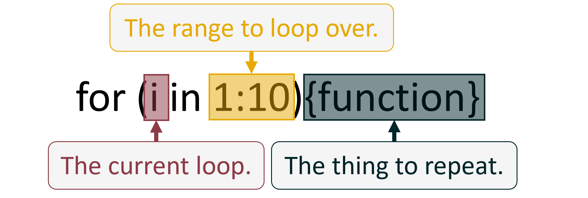
[1] 10

In this simple (very unrealistic) example it seems pretty straight forward, but I think we can explain things a bit more. The “For Loop” is usually denoted like this; for (i in n){f} where:

• “i” is the iteration (or current loop)
• “n” is the range to loop over
• “f” is the function or functions to loop over

For Loop

Everything that isn’t highlighted is just the syntax of the for loop, but that doesn’t mean it isn’t also important to understand. Case and point, these next two code chunks will execute identically and produce the same results, even if they look a bit different.

#write a for loop to print the numbers 1 to 10
for (i in 1:10){print(i)}

#write a for loop to print the numbers 1 to 10
for (i in 1:10){
  print(i)
}

From now on I will be writing our for loops using the second format because I think it is easier to follow, but just remember that this doesn’t change how the code runs just how it looks. Time to dive in!

2.1 i The Iteration

“i” can be anything, which is not super helpful (sorry). What might be helpful is just seeing an example. This code:

#write a for loop to print the numbers 1 to 10
for (PotatoSalad in 1:10){
  print(PotatoSalad)
}

will produce the exact same result as this code:

#write a for loop to print the numbers 1 to 10
for (i in 1:10){
  print(i)
}

We use “i” as an iteration counter (hence usually getting called “i”) that keeps track of what loop we are on with respect to n. For our example above, n is 10. So on the first loop “i” is 1, on the second loop “i” is 2, on the third loop “i” is three…, all the way until “i” is 10. At that point, the for loop finishes. Hopefully it is now intuitive to see how print(i) produces the numbers it does.

2.2 n The Range

“n” is the range of the loop. “n” tells the for loop two things;

1. How many times to continue looping
2. What elements to loop over

In our example above, n is 10. But wait, that’s not quite right, n is actually 1 to 10. This is an important distinction to make because it is usually one of the first places we make errors. Lets take a look:

#write a for loop to print the number 10 (spot the issue)
for (i in 10){
  print(i)
}

[1] 10

As you can see, when “n” is just 10, then the output is only the value “10”. This is because the range (AKA length) of “n” was only 1. An easy way to check this is to use the length() function:

length(10)

[1] 1

length(1:10)

[1] 10

So the first super important thing to remember is that “n” is a range, it has a point you want to start at, and a point you want to end at. The second super important thing to remember about “n” is that it directly tells the specific value to start and end at, and therefore determine the value that “i” is going to be. Here is a simple demonstration:

#write a for loop to print the numbers 15 to 22
for (i in 15:22){
  print(i)
}

[1] 15
[1] 16
[1] 17
[1] 18
[1] 19
[1] 20
[1] 21
[1] 22

In this case, we started at 15 and ended at 22. So on the first loop, “i” is 15, second loop “i” is 16, etc.

The last super important thing to remember about “n” is that it does not have to be numeric! It took me a while to realise this, but it can allow you to do some cool things. Here is another quick example:

#create a vector of character elements
n_range <- c("PotatoSalad", "FishFingers", "Im... Kinda Hungry")

#write a for loop to print this vector one element at a time
for (i in n_range){
  print(i)
}

[1] "PotatoSalad"
[1] "FishFingers"
[1] "Im... Kinda Hungry"

This does throw a minor curve ball though. Did you notice that the code is now for (i in n_range), there is no “1:” in front of “n_range”, this is just because the object “n_range” already has a range of elements that we can loop over. Lets use length() again to show this:

length(n_range)

[1] 3

If you can remember these core things about for loops you will get very, very far with them. So to summarise. “n”:

• Must be a range, it needs a start and end point
• Tells “i” what value it is going to be
• Can be a numeric, or character!

2.3 f The Function

The final part of a for loop is by far the biggest part of the code, but it is ironically very straight forward to understand if you have a little bit of an R background. The function or functions inside a for loop are the exact same functions that you would be using outside a for loop! The hard part to figure out is where to place that stupid “i” value. Personally, I haven’t been able to find a method of explaining where “i” goes other than by being very conscious of the purpose of your for loop. Start with simple and short loops and work your way to more complicated tasks, it will come naturally. Generally you will find that “i” only needs to be placed in a few key locations, however if you miss a spot, happy debugging!

Note

Want to learn more about For Loops from the professionals? Check out the Iteration chapter in R for Data Science!

3 For Loops in Action

So far all I have done is demonstrate a very silly example of a for loop. The kind of example that really doesn’t give you a compelling reason to learn how to write a for loop. The kind of examples I used to read that made me not bother learning for quite a while. So instead of demonstrating a million more half baked for loops lets just cut to chance and see how I implement a for loop in my day to day. (If this blog post does compel you to go on the learning journey - the link above will fill the gaps in what I’ve written )here.

3.1 The Scenario

Something I do almost every day is make maps. Usually fairly simple maps, often they show sample site locations, or coral monitoring locations, or the size of a seagrass meadow, things like that. These maps are included in static word documents and are often needed over large chunks of areas. However, the combination of a large study location, a high quantity of sample site locations, and a static output (can’t put an interactive map into word), means that instead of one large map, I need to create lots of small maps for each little area.

This here, is an absolutely prime example of a compelling reason to use a for loop. To give you some numbers, in one of my projects I need to create 67 maps. If I was to manually write out the code for each of those 67 maps, my script would have 3886 lines of code just dedicated to creating the maps. Instead, I use a for loop and pull 67 maps out of less than 100 lines of code. Not only that, but I also reduce the chance of an error sneaking into my code by 67x.

Below is a simplified mock up of the code I would use for this, noting that I have used made up sampling locations for data privacy, and created interactive maps for your enjoyment. We will see the full code in action first, then break it down step by step.

#read in some example data that I made up
example_sites <- st_read("example_data.gpkg")

#extract an object that contains the three unique locations we are looking at
locations <- unique(example_sites$Location)

#create a list that will store my maps
list_of_maps <- setNames(vector("list", length(locations)), locations)

#initialize the for loop
for (i in locations){
  
  #filter our dataset
  sub_set_of_sites <- example_sites |> 
    filter(Location == i)
  
  #create a simple map
  single_map <- tm_shape(sub_set_of_sites) +
    tm_dots(shape = "Site", size = 1, col = "Site", fill = "Site") +
    tm_text("Site", size = 2, ymod = 1) +
    tm_layout(legend.show = F)
  
  #add each map to the list
  list_of_maps[[i]] <- single_map
  
}

Here is how one of the maps looks:

#view the map
list_of_maps[["Alligator Creek"]]

3.2 The Breakdown

Time to take a closer look at whats happening here.

1. First of all, i use a function called st_read() from the sf package to load in my dataset. For the purposes of this post, we don’t need to worry about this package and its functions. Check out my other posts for more details on this area. What I will do here though, is show a sneak peak of the data.

#read in some example data that I made up
example_sites <- st_read("example_data.gpkg")

Location	Site	X	Y
Alligator Creek	Site 1	147	-19.3
Alligator Creek	Site 2	147	-19.3
Alligator Creek	Site 3	147	-19.3
The Strand	Site 1	147	-19.2
Town Common	Site 1	147	-19.2
Town Common	Site 2	147	-19.2
Town Common	Site 3	147	-19.2
Magnetic Island	Site 1	147	-19.2
Magnetic Island	Site 2	147	-19.2

2. From this dataset I then extract a vector of unique locations, which in this case we can easily see is just the four (Alligator Creek, The Strand, Town Common, Magnetic Island).

#extract an object that contains the three unique locations we are looking at
locations <- unique(example_sites$Location)

3. I then create a list to store the outputs of my for loop. This step can be done in a wide range of ways, for example you could store each output as a separate object, if you know the number of outputs you could pre-define a list of that length to store the outputs (like I did), or if the number of outputs is a mystery you can grow the list as you go. There is no “best” way to do this, however it is generally frowned upon to grow the list as you go, as this can be computationally quite expensive. My recommendation would be to use the first two options, favoring a list with a pre-defined length if you can.

#create a list that will store my maps
list_of_maps <- setNames(vector("list", length(locations)), locations)

4. The set up is done and it is now time to begin the for loop. This section of the code is a good time to review what we discussed above. We can see that I am going to loop over “locations”, and for each loop “i” will become of the elements in “locations”.

#initialize the for loop
for (i in locations){

5. We are now working within the for loop. Remember, this section of the code will be run again and again and again. The first thing we do inside the for loop is take a subset of our data. We can filter the data by “i” because “i” has taken on the first element of “location”.

  #filter our dataset
  sub_set_of_sites <- example_sites |> 
    filter(Location == i)

6. Using the subset of the data, which will now only contains rows from one location thanks to our filter. We then create the map. I like to use the tmap package, however there is a wide range of options available. Maybe I will write a post on mapping with tmap one day… we will see.

  #create a simple map
  single_map <- tm_shape(sub_set_of_sites) +
    tm_dots(shape = "Site", size = 1, col = "Site", fill = "Site") +
    tm_text("Site", size = 2, ymod = 1) +
    tm_layout(legend.show = F)

7. The final step of our for loop is to save the output of the loop somewhere. This step can catch alot of people off guard, they write the perfect loop, they check everything runs properly, and then they forgot to save the output each loop. Shame.

In my case, I have put the map into the list that we defined earlier. Notice that because I named each item in the list, I can then place the map under the correct item using “i”.

  #add each map to the list
  list_of_maps[[i]] <- single_map
  
}

4 Writing Your Own For Loop

To start writing your own for loops all you really need to do is start giving it a crack. Although, I do remember starting the journey and having trouble finding good opportunities. Here are hopefully some good points to get you going:

• Don’t try to create the worlds most complicated for loop on your first go, start small.
• Look for places in your script that you have copied the same code, even a single repeat of code is an opportunity to practice a loop.
• Is there a part of your script that breaks down something big to do something small. You could loop that small thing and do it more times!
• Screw legit opportunities, why not just try: - make 100 copies of the same table to fk with your boss. - create a loop that grows an objective to a length of 100million and break your computer. - put a loop inside a loop and see what happens (this one doesn’t break your computer btw).

Once again, I will link to the Iteration chapter in R for Data Science as this is the most comprehensive place to go for learning something new in R the right way.

5 Caveats

As always, I like to finish my posts with an acknowledgement of caveats. With respect to this post, please remember to take a random internet stranger’s opinion with a grain of salt, refer to the linked educational resources, and think critically about the things you are learning and if they make sense to you. With respect to for loops, don’t over do it with your new power! It is often cleaner and simpler to write two or three separate for loops rather than one complicated one. You can even sometimes cause memory overflows and crash your computer when writing loops for large datasets and using poor memory management techniques.

Finally, the thing I have been alluding to this entire time, as of writing this post I currently try my best to avoid using for loops! Instead, I have been progressing in my journey of learning to use vectorised functions. To find out how you can take the next step from for loop to vectorised function, check out this Loops and Vectorised Functions blog post!