Multiple Linear Regression Modelling in R

1 Introduction

Today I’d like to discuss multiple linear regression. What is it? What can we use it for? How should the results be interpreted? How can we actually implement it in R? I’ll be answering all of these questions and more!

Just as a quick recap, In a previous blog I wrote about using simple linear regression to predict tree height based on elevation (a completely made-up relationship). Before reading this blog I encourage you to take a look at that post as it covers some of the more basic aspects of modelling.

Ideally, by the end of this series we are both able to explain in more detail exactly what we are doing to our colleagues.

2 Multiple Linear Regression

You might recall that linear regression uses the equation:

\(y = slope*x + y-intercept\)

It is sometimes also written as \(y = mx+b\) or as \(y_{i} = f(x_{i},\beta) + e_{i}\)

All of these mean the same thing despite their varying levels of stupidly confusing mathematical symbols. In every case:

• \(y\), \(y\), or \(y_{i}\) means “the dependent variable”
• \(y-intercept\), \(b\), or \(e_{i}\) means “where does the line cross the y-axis”, and
• \(slope*x\), \(mx\), or \(f(x_{i},\beta)\) all just mean “the independent variable (x) multiplied by some constant”

The equation simply represents the line that best fits all of the points in a dataset. Where the dataset contains one indepent variable (x) and one dependent variable (y). The idea of linear regression is two fold:

1. Establish if there is a relationship between x and y, and
2. Use the equation to predict unknown y values based on known x values

Multiple linear regression is the natural extension of this equation. The only thing that changes is there is now additional independent variables. The equation for multiple linear regression looks like this:

\(y_{i} = \beta_{0} + \beta_{1}*x_{i,1}+\beta_{2}*x_{i,2}+...+\beta_{n}*x_{i,n}\)

Again, I’ll just acknowledge that mathematicians must have been on crack when they decided how to write these things. Anyway, it is essentially the same thing as above, there are now just more independent variables. Some important notes about this equation:

• We are always trying to predict y. No matter how fancy the right side of the equation is, just remember we are predicting y
• To predict y we input several independent variables, these are the \(x_{i,n}\) terms.
  • The “i” in this just means that each group of independent variables we plug in will return 1 y value - note there is also an “i” over on the left side of the equation. (This makes sense later)
  • The “n” is just signifying that each “x” is unique. Note in the full equation how the first “x” is 1, then the second “x” is 2 and so on. This is important because it signifies that each of the x terms is going to be different.
• The \(\beta_{1}\) terms are the constants that are applied to each independent variable. Note that these values also have numbers associated with them, it signifies that each one is matched up to a specific independent variable and each one will be different.
• The y-intercept has been replaced with \(\beta_{0}\) however the idea is still the same, it just looks more “mathy” now.

Enough of that boringness though, lets get right into things. To do this I’m going to create a hypothetical dataset for us to practice on. This dataset is going to look at mouse weight as a factor of body length and tail length.

2.1 Building A Dataset

The first thing we need to do is build a dataset that explores this relationship between mouse weight, body length and tail length. I am going to manually create 50 of each of these values. Note that we want to show a relationship so I will deliberately try to add a trend, however to make things interesting I will make sure it is not a completely perfect reationship. We will achieve this by asking for random numbers between 0g and 1000g for weight, 0cm and 30cm for the body, and 0cm to 25cm for the tail. Then each of these will be ordered smallest to largest to create a trend:

Note

I will say that the total length of the mouse is body + tail.

#load libraries
library(tidymodels)
library(gt)

set.seed(123)

#create each variable
body_length <- runif(50, 0, 30)
tail_length <- runif(50, 0, 25)
weight <- runif(50, 0, 1000)

#make a dataframe
mouse_df <- data.frame(
  Weight = weight[order(weight)],
  BodyLength = body_length[order(body_length)],
  TailLength = tail_length[order(tail_length)])

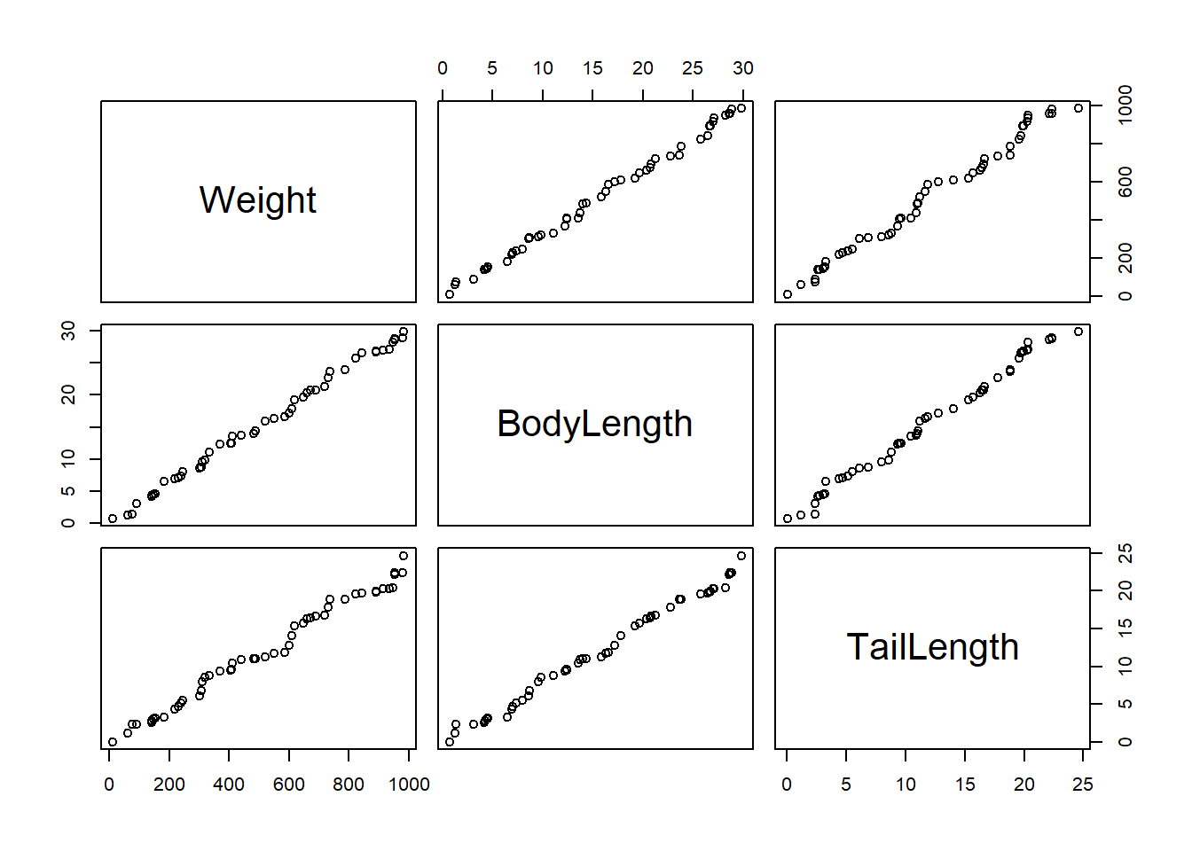
On a plot, this is how our make believe data looks, obviously the trends are pretty easy to spot since we specifically created the data for this purpose:

#create a simple plot to show the data pointsw
plot(mouse_df)

However something to note here (that is particularly important when doing this type of analysis for real) is that the two independent variables (body length and tail length) seem to also be highly correlated - aka collinearity. This can introduce problems in your model for a few reasons:

• redundant information, which can confuse the model and also impose limitations on the data you might be able to collect/use
• large swings in coefficent estimates, i.e. a small change in the data can wildly change the estimate
• difficulty interpreting effects, if the two variables change together it can be hard to determine which variable is a greater factor

You can address collinearity in a few different ways:

• If it is mild you could ignore it,
• If it affects variables you are not going to use in the final model you can also ignore it (also if it affects control variables - I’m not sure I understand that one yet)
• If you are using the model for predictions, rather than to find statistically significant independent variables, you can also ignore collinearity. The reason being that it does not inhibit our ability to obtain a good fit nor does it tend to affect inferences about mean responses or predictions of new observations.
• If you can’t ignore it, you can consider removing offending variables, combining them together, or using more advanced statistical methods I won’t be covering here. - In any case, If you’re stuck the first thing I’d reccomending is seeking more experienced advice

Our objective in this blog is to simply learn about multiple regression, plus make some predictions… So I going to ignore it :)

2.2 Building A Multiple Regression Model

Making a multiple regression model is very straight forward in R - if you use the right set of packages. Following on from my first modelling blog, I am going to be leveraging the tidymodels() package, which is actually a wrapper for a collection of packages that do a wide range of things within the modelling ecosystem such as preparing data, creating models, and evaluating model performance. Thanks to this collection of packages the model creating process is reduced to three simple steps:

1. Define the model to be used (for us this is a linear regression)
2. Define the “engine” that runs the model (for us there is only one option “linear model”, but for more complex models there are multiple methods of implementation)
3. Fit the model, i.e. input the required variables (the dependent variable is mouse weight, and our two independent variables are body length and tail length)

Note

When you are using “real” data that wasn’t made up for educational purposes there are extra steps in the model building stage focused on properly preparing the data such as removing colinearity and normalising numeric data to have a standard deviation of one. But we are not going to cover those in this example.

Note

Interestingly, for a lot of models (not just linear regression) made using tidymodels packages, these general steps are almost the same. You can swap out a different model and engine while keeping the same inputs if you wanted.

The code to create our multiple regression model is as follows:

#create a linear model based on the example data
my_lin_mod <- linear_reg() |> #set up the framework
    set_engine("lm") |> #choose the linear model method as the "engine"
    fit(Weight ~ BodyLength + TailLength, data = mouse_df) #dependent ~ independent(1) + independent(2) + ..., define the dataset

Next, to view the model that we just created we can use the tidy() function to return a nice layout:

#get a nicer view of the information inside the object
gt(tidy(my_lin_mod))

term	estimate	std.error	statistic	p.value
(Intercept)	-3.328716	6.041809	-0.5509469	5.842797e-01
BodyLength	34.270229	3.492987	9.8111535	5.903997e-13
TailLength	-1.340849	4.458381	-0.3007479	7.649331e-01

Which, on its own, it is not really anything special - just a table. But intepreting the table can allow us to understand a bit about the multiple regression model that we just created.

• The intercept estimate is the y-intercept (where the regression line crosses the y axis)
• The BodyLength estimate is the constant that is applied to the BodyLength input value
• The TailLength estimate is the constant that is applied to the TailLength input value - i.e. in the equation earlier these are the \(\beta_{1}\) values
• Together, these define the equation of the regression line, which would be: y(pred) = -3.33 + 34.27\(x_{BodyLength}\) + -1.34\(x_{TailLength}\)

Unfortunately, unlike with the simple linear model, it is not easy to then visualise this equation in a graph. Thats because we are now dealing with two independent variables, and would thus need two axis to show the changes across both of these variables - resulting in a 3D graph. Furthermore, if you added a third independent variable, that equates to another dimension, a forth variable equals another dimension, and so on.

For now, we can actually produce a 3D graph to explore our data, but generally from this point onwards the way we try to visualise our data/model is going to have to change.

First up, here is just the points in space, I’ve made this plot interactive so you can get a good understanding of the data:

library(plotly)

#plot the points in 3D space
plot_ly() |> 
  add_markers(
    data = mouse_df, 
    x = ~BodyLength, 
    y = ~TailLength, 
    z = ~Weight,
    marker = list(
      size = 4,
      color = "#8E3B46")) |> 
  layout(scene = list(
    xaxis = list(title = "Body Length (x-axis)"),
    yaxis = list(title = "Tail Length (y-axis)"),
    zaxis = list(title = "Weight (z-axis)")
  ))

To add the multiple regression equation to this graph we are going to have to do a bit of thinking. If we consider the simple linear model again, the way we added the equation was basically by giving the simple linear model two points of data, predicting the results based on each point of data, and then drawing a line on the graph between the two. However, if we:

1. Give the model some mouse body length and tail length values,
2. Predict some weight values based off this information
3. Then plot these new points:

#create a dataframe of new lengths to predict weight from
line_data <- data.frame(BodyLength = c(0, 5, 15, 30), TailLength = c(0, 5, 20, 25))

# Predict weight based on this data
line_data <- my_lin_mod |> 
    predict(line_data) |> 
    bind_cols(line_data)

#plot the points in 3D space and add the prediction line based on the four predictions
plot_ly() |> 
  add_markers(
    data = mouse_df, 
    x = ~BodyLength, 
    y = ~TailLength, 
    z = ~Weight,
    name = '"Real" Mouse Weights',
    marker = list(
      size = 4,
      color = "#8E3B46")) |> 
  add_trace(
    data = line_data, 
    x = ~BodyLength, 
    y = ~TailLength, 
    z = ~.pred,
    name = "Predicted Mouse Weights",
    line = list(
      color = "#00252A", 
      width = 1),
    marker = list(
      size = 2,
      color = "#00252A")) |> 
  layout(scene = list(
    xaxis = list(title = "Body Length (x-axis)"),
    yaxis = list(title = "Tail Length (y-axis)"),
    zaxis = list(title = "Weight (z-axis)")
  ))

The line looks kind of strange, it’s bent, and doesn’t clearly represent the “line of best fit”. This is because in a multiple regression model we are no longer getting the line of best fit, but a higher dimensional object of best fit, in this case it is a plane, but with extra independent variables I’m not even sure what it is called. (Once again another reason that visualising the model starts to breakdown at this point).

The solution to this is that we need to visualise the entire “plane-of-best-fit” to see exactly where each prediction will land. To do this we need to create a grid of all possible points within the space, calculate a prediction for all of those points, then plot those points as a plane:

#sequence from the smallest body length to the largest, increaes by 0.05cm each time
body_length_vals <- seq(min(mouse_df$BodyLength), max(mouse_df$BodyLength), by = 0.05)

#sequence from the smallest tail length to the largest increaes by 0.05cm each time
tail_length_vals <- seq(min(mouse_df$TailLength), max(mouse_df$TailLength), by = 0.05)

#build a grid based off every combination of these values
grid <- expand.grid("BodyLength" = body_length_vals, "TailLength" = tail_length_vals)

#predict the weight based on this grid of values
grid_predictions <- my_lin_mod |> 
    predict(grid)

#convert the prediction values into a matrix, the dimensions of the matrix are based on the original indepedent variables
plane_o_b_f <- matrix(
    data = grid_predictions$.pred,
    nrow = length(body_length_vals), 
    ncol = length(tail_length_vals), 
    byrow = FALSE)

#and transpose the matrix to the correct orientation
plane_o_b_f <- t(plane_o_b_f)

#plot the points in 3D space and add the prediction plane
plot_ly() |> 
  add_markers(
    data = mouse_df, 
    x = ~BodyLength, 
    y = ~TailLength, 
    z = ~Weight,
    marker = list(
      size = 4,
      color = "#8E3B46")) |> 
  add_surface(
    x = ~body_length_vals,
    y = ~tail_length_vals,
    z = ~plane_o_b_f,
    showscale = FALSE,
    opacity = 0.8,
    name = "Prediction Plane",
    colorscale = list(c(0, "#00252A"), c(1, "#E6AA04"))) |> 
  layout(scene = list(
    xaxis = list(title = "Body Length (x-axis)"),
    yaxis = list(title = "Tail Length (y-axis)"),
    zaxis = list(title = "Weight (z-axis)")
  ))

Pretty cool. Note how the plane seems to split right down the middle of all our datapoints, the closer the plane is to all the points, the better our model is “fitted” to the data. Speaking of model fit, we can now look at the “fit” (i.e. the accuracy) of our model by the numbers!

2.3 Evaluating a Multiple Linear Regression Model

The performance of a linear model can be evaluated several ways, and we are going to touch on pretty much all of them. Firstly lets bring up the tabular summary of the model again:

#re print the tabular summary of the model
gt(tidy(my_lin_mod))

term	estimate	std.error	statistic	p.value
(Intercept)	-3.328716	6.041809	-0.5509469	5.842797e-01
BodyLength	34.270229	3.492987	9.8111535	5.903997e-13
TailLength	-1.340849	4.458381	-0.3007479	7.649331e-01

Looking at the table again there are a few additional columns to cover, these speak to the accuracy of the regression.

• The std.error column is the standard error of the estimate, with smaller values indicating greater precision. You can think of this as how far each of the observations are from the regression equation (aka the plane-of-best-fit we looked at before).
• The statistic is the estimate divided by the std.error. In this case large values are often a case for some kind of statistical significance (that is to say that the std.error is much smaller than what ever the estimate value is).
• The p.value is the one familar to most introductory statistics students, and represents the likelihood of randomly observing the slope (estimate for dependent variable - e.g. mouse body weight). I.e. if tail length or body length had no real effect on mouse body weight (slope of the regression line = 0), then the chances of getting a slope as large as 34.27 just from random noise are about 0% (for Body Length), and the chances of getting a slope as large as -1.34 just from random noise are about 0.76% (for Tail Length).
  • Generally, a p-value of less than 0.005 is considered to be a significant effect.

So why is the first row not significant? Well the first row is talking about the intercept. It is saying, is the intercept statistically different from 0? I.e., when body length and/or tail length is 0, is a mouse weight of of -3.33g any more or less likely than a mouse with a weight of 0g? The answer is no (because the p value is high (>0.05) and the statistic is low we don’t have any strong evidence to disprove this). Conversely, the second row the table is talking about the slope (with respect to BodyLength - i.e. only changing the body length value and keeping tail length constant). It is saying, is the slope significantly different from 0? (zero being no relation) I.e. Does mouse weight change with body length? The answer is yes - because the p value is low (<0.05) and the statistic is high we have strong evidence to disprove the null hypothesis. Further more, because the slope is positive, not negative, we can say that mouse weight increases with body length. This same observation can be made about tail length.

Note

There are additional methods for evalutation the performance of our model, but we will explore these further into the blog.

2.4 Using a Multiple Regression Model

Now that we have established our multiple regression model is not useless, what is the point of the model, and how do we use it? Well point 1 is simply to be able to confirm “yes, mouse weight does change with body length and tail length”, congratulations we can all go home. But that is kind of boring and doesn’t have a satisifying conclusion, particularly because we specifically made this data up to have that relationship. Point 2 is that we can use this model to predict the weight of mice that we have never weighed before.

Imagine that the data I just made up is from a group of mouse from Pet Store A, and on the other side of the city is a second store; Pet Store B:

Unfortunately this pet store is very small, and doesn’t have the funds to own a scale to weigh mice on. Thankfully, due to the data we obtained from Pet Store A, we can simply ask Pet Store B to measure the body and tail length of their mice and we will be able to calculate the weight of each mouse with pretty good accuracy.

This is acheived using the predict() function from the tidymodels group of packages. To use predict, obviously I need to create some new mouse data for Pet Store B for us to predict on, so I will also do that here.

#create random body length values, multiple by 29 rather than 30 to add some variation compared to Store A
body_length_b <- runif(15, min(mouse_df$BodyLength), max(mouse_df$BodyLength))

#create random tail length values, multiple by 29 rather than 30 to add some variation compared to Store A
tail_length_b <- runif(15, min(mouse_df$TailLength), max(mouse_df$TailLength))

#create another set of fake data, this time its is the body and tail lengths of mice from Pet Store B, it will not contain any mouse weight information - we are going to predict that
store_b_data <- tibble(
  BodyLength = body_length_b[order(body_length_b)],
  TailLength = tail_length_b[order(tail_length_b)])

#use the linear model to predict values
store_b_output <- my_lin_mod |> 
    predict(store_b_data) #note that the column names must match what was used in the model

#view the output
gt(store_b_output)

.pred
281.1279
278.2926
284.6677
320.1553
379.6199
486.3648
533.1605
565.8994
582.0657
594.0053
706.3056
830.0842
863.0079
889.2895
899.8002

The output of the predict function is provided as a table (specifically a tibble), rather than a vector, because a common next step with the predicted values is to join them back to the original independent values. Thus we will do that now:

#add the columns from the original dataset onto the predicted values
store_b_output <- store_b_output |> 
    bind_cols(store_b_data)

#update the column name of the data
store_b_output <- store_b_output |> 
  rename(PredictedWeight = ".pred")

#view the data
gt(store_b_output)

PredictedWeight	BodyLength	TailLength
281.1279	8.447694	3.764611
278.2926	8.448129	5.890262
284.6677	8.713831	7.926765
320.1553	9.827429	9.922267
379.6199	11.566698	10.027080
486.3648	14.738978	11.496198
533.1605	16.151163	12.689628
565.8994	17.162167	14.112907
582.0657	17.661336	14.814211
594.0053	18.027666	15.272604
706.3056	21.342351	16.238160
830.0842	25.166988	21.676995
863.0079	26.182642	23.081330
889.2895	26.973650	23.697642
899.8002	27.302766	24.270571

And just like that we have now predicted (with pretty good accuracy) the weights for each mouse that Store B has, without ever having gone to that store, or the store having their own scales! Thats fun.

Also here is a visualisation of the new data combined with the old data. Something that might not be clear until seeing this that each of the predictions land exactly on the plane of best fit. This is because the math that calculates the plane is the same math used to predict the mouse weights:

#plot the original data, the plane of best fit from the linear model, and the predicted data
plot_ly() |> 
add_markers(
    data = mouse_df,
    x = ~BodyLength,
    y = ~TailLength,
    z = ~Weight,
    name = '"Real" Mouse Weights',
    marker = list(
      size = 4,
      color = "#8E3B46")
  ) |> 
add_markers(
    data = store_b_output,
    x = ~BodyLength,
    y = ~TailLength,
    z = ~PredictedWeight,
    name = "Predicted Mouse Weights",
    marker = list(
      size = 4,
      color = "#E6AA04")
  ) |> 
  add_surface(
    x = ~body_length_vals,
    y = ~tail_length_vals,
    z = ~plane_o_b_f,
    showscale = FALSE,
    opacity = 0.8,
    name = "Prediction Plane",
    colorscale = list(c(0, "#00252A"), c(1, "#E6AA04"))) |> 
  layout(scene = list(
    xaxis = list(title = "Body Length (x-axis)"),
    yaxis = list(title = "Tail Length (y-axis)"),
    zaxis = list(title = "Weight (z-axis)")
  ))

What probably comes to mind looking at this is “how accurate is this plane?” Yes we know that the model proved there was a significant relationship between mouse weight and tail length, and mouse weight and body length, but how strong is the relationship? How accurate is that plane on the graph?

An easy way to test the accuracy of the model is to have some training data, and some testing data. Training data is data used to train the model. This data is like the red dots on our graph, for each data point we know the weight of the mouse, the length of the mouses’ body, and the length of its tail. The training data is shown to the model, and the linear regression model is created. Testing data is additional data that we withhold from the model.

Note that in the testing dataset we also know both the weight of the mouse, as well as the tail length and body length of the mouse. Generally, training data and testing data come from the same parent dataset, and each group is created randomly. The training dataset normally receives about 80% of the total data, and 20% of the data is withheld for testing, however the split could be whatever you want - if you can justify it.

To split the dataset into testing and training we can use the initial_split() function:

#create a split of the data
mouse_split <- initial_split(mouse_df)

Note that the output of this is no longer just a df, it is a rplit object. When looking at it you can see the division of rows:

#view object
mouse_split

<Training/Testing/Total>
<37/13/50>

To access specifically the training or testing data from this object you can use the training() or testing() functions:

#to see the training or testing part of the data, use training() or testing()
mouse_split |> 
    testing() |> 
    gt()

Weight	BodyLength	TailLength
76.69117	1.366695	2.339875
141.90691	4.164182	2.571616
239.09996	7.382632	5.163285
307.72001	8.674792	6.859591
319.82062	9.837622	8.587912
409.47495	12.436390	9.599241
619.25648	19.215204	15.319275
690.00710	20.784102	16.627880
821.80546	25.734831	19.557358
842.72932	26.490522	19.704896
890.35022	26.686179	19.858558
954.09124	28.635109	22.161727
984.21920	29.828093	24.623924

With our dataset split we can the create a new linear model the same way we did before, but this time we are only going to show it 80% of the data (the training data):

#train a new model on just the training data
new_lm <- linear_reg() |> 
  set_engine("lm") |> 
  fit(Weight ~ BodyLength + TailLength, data = training(mouse_split))

#view new model
gt(tidy(new_lm))

term	estimate	std.error	statistic	p.value
(Intercept)	-13.590197	7.340279	-1.851455	7.280575e-02
BodyLength	40.109312	4.580044	8.757407	3.109156e-10
TailLength	-8.131044	5.818958	-1.397337	1.713651e-01

With the new model trained, we can now use it to predict values based on the testing data. Remember that in this case we know the real mouse weight as well as the mouse body length and tail length (this) varies from the scenario above with Store B where we only knew the mouse body length and tail length). The goal of predicting on mice that we already know the weight for is to see how close we get to the real answer:

#test new model on just the testing data
testing_output <- new_lm |> 
    predict(testing(mouse_split)) |> #use model to predict weight based on tail and body length
    bind_cols(testing(mouse_split)) #bind the full testing dataset on to the predicted outputs

gt(testing_output)

.pred	Weight	BodyLength	TailLength
22.20138	76.69117	1.366695	2.339875
132.52235	141.90691	4.164182	2.571616
240.53920	239.09996	7.382632	5.163285
278.57411	307.72001	8.674792	6.859591
311.16135	319.82062	9.837622	8.587912
407.17301	409.47495	12.436390	9.599241
632.55674	619.25648	19.215204	15.319275
684.84383	690.00710	20.784102	16.627880
859.59446	821.80546	25.734831	19.557358
888.70505	842.72932	26.490522	19.704896
895.30330	890.35022	26.686179	19.858558
954.74638	954.09124	28.635109	22.161727
982.57590	984.21920	29.828093	24.623924

Looking at the table, the .pred column is the models predictions based on the mouses’ tail length and body length, and the Weight column is the actual weight of the mouse that was measured with those specific tail and body lengths. The model does seem to be broadly correct, but how correct? Thankfully the tidymodels package also gives us an easy way to compare the predicted values against the true values using the metric() function:

#you can see accuracy metrics using the metrics() function
testing_output_metrics <- testing_output |> 
    metrics(truth = Weight, estimate = .pred)

gt(testing_output_metrics)

.metric	.estimator	.estimate
rmse	standard	24.4352191
rsq	standard	0.9967585
mae	standard	16.5308068

Okay cool, but what do these values actually mean?

• RMSE is Root Mean Square Error, it is the average difference between the predicted values and the actual values. So for us, it is saying our model is on average 24.44 grams from the real value.
• RSQ is “R Squared”, it tells us as a proportion how much of the variance in the dependent variable is predictable from the independent variables. In our case it is saying our model can explain 99.68% of the variance in mouse weight using mouse body and tail length. Nice!
• MAE is Mean Absolute Error, it is also looking at the average distance between the predicted and actual values, but it is not squaring this number (which RMSE does). In a nutshell this make RMSE very sensitive to large errors, but MAE treats all errors equally. In our case, the MAE is saying our model is on average 16.53 grams from the real value. This is a fairly similar value to RMSE and thus also tells us that there are not any particularly large errors distorting the average error.

3 Extending the Linear Model

So far we have only looked at modelling values within the original bounds of our training dataset. By that I mean, in our training data mouse weight ranged from 0g to 1000g, and when we have predicted values, we have only predicted values for elevations from 0g to 1000g. So what happens if we look further afield?

Let’s pretend there is a third pet store; Store C. This store stocks a particular breed of mouse that is huge, some of their mice have tail lengths of 50cm! Could we use our model to try and predict mouse weights at this store? In theory yes, but there are important caveats and precautions that need to be taken. Let’s take a look.

#create store C data, values must be ordered so that body and tail length are related, lengths go up to 50cm
store_c_data <- data.frame(
  BodyLength = sort(runif(50, 10, 45)),
  TailLength = sort(runif(50, 15, 50))
)

#use the linear model to predict values
store_c_output <- my_lin_mod |> 
    predict(store_c_data) |> #note that the column name must match what was used in the model
    bind_cols(store_c_data)

#rename the column
store_c_output <- store_c_output |> 
  rename(PredictedWeight = ".pred")

#view the output
gt(store_c_output)

PredictedWeight	BodyLength	TailLength
339.2565	10.62180	15.97974
458.6100	14.17917	17.88760
478.5785	14.77891	18.32368
487.0207	15.03360	18.53705
509.9096	15.70746	18.68962
545.0018	16.74856	19.12698
544.7779	16.76825	19.79736
562.2682	17.31067	20.61663
580.5310	17.87757	21.48538
585.2188	18.02357	21.72082
678.9592	20.78418	22.36705
679.5397	20.80754	22.53102
684.9713	20.99948	23.38581
694.4030	21.31707	24.46907
717.4907	21.99831	24.66174
741.7802	22.71552	24.87764
749.4126	22.95752	25.37058
770.8181	23.59117	25.60167
792.0956	24.23128	26.09322
801.6200	24.51574	26.26039
806.6244	24.66206	26.26781
809.3223	24.76457	26.87594
847.6527	25.92878	28.04483
880.5818	26.91087	28.58716
884.1330	27.02441	28.84071
888.9646	27.23983	30.74309
914.6140	28.02751	31.74597
926.8427	28.41104	32.42821
934.2564	28.68177	33.81870
995.1318	30.47150	34.16108
1038.7549	31.76658	34.72756
1039.8344	31.81541	35.17056
1060.6855	32.45118	35.86922
1062.2293	32.53730	36.91899
1091.1902	33.40700	37.54841
1123.7822	34.40808	38.82756
1171.0619	35.82291	39.72757
1197.7667	36.62883	40.40941
1212.2528	37.11070	41.92179
1222.6996	37.43813	42.49907
1280.6487	39.19190	44.10490
1280.6352	39.23394	45.18932
1316.7515	40.32692	46.18900
1352.3753	41.38585	46.68584
1432.4569	43.73452	46.98984
1435.0875	43.86143	48.27174
1439.6166	43.99699	48.35854
1446.3000	44.22487	49.19846
1452.4729	44.41726	49.51190
1455.3530	44.50840	49.69328

So far so good, for this plot we will also need to extend the plane of best fit a bit further:

#sequence from the smallest val to the largest, increasing by 0.05 each time
body_length_vals_2 <- seq(min(store_c_output$BodyLength), max(store_c_output$BodyLength), 0.05)
tail_length_vals_2 <- seq(min(store_c_output$TailLength), max(store_c_output$TailLength), 0.05)

#combine these values in every possible way to create pairwise combinations
grid <- expand.grid("BodyLength" = body_length_vals_2, "TailLength" = tail_length_vals_2)

#predict weights based on every pair
grid_predictions <- my_lin_mod |> 
  predict(grid)

#convert the predicted values from a single row into a matrxi with the dimensions of the original data
plane_o_b_f_2 <- matrix(
  data = grid_predictions$.pred,
  nrow = length(body_length_vals_2),
  ncol = length(tail_length_vals_2)
)

#and transpose the matrix to the correct orientation
plane_o_b_f_2 <- t(plane_o_b_f_2)

and here is the plot:

#plot the original data, the plane from the linear model, and the predicted data
plot_ly() |> 
  add_markers(
    data = mouse_df,
    x = ~BodyLength,
    y = ~TailLength,
    z = ~Weight,
    name = '"Real" Mouse Weights',
    marker = list(
      size = 4,
      color = "#8E3B46"
    )
  ) |> 
  add_markers(
    data = store_c_output,
    x = ~BodyLength,
    y = ~TailLength,
    z = ~PredictedWeight,
    name = "Predicted Mouse Weights",
    marker = list(
      size = 4,
      color = "#E6AA04"
    )
  ) |> 
  add_surface(
    x = ~body_length_vals,
    y = ~tail_length_vals,
    z = ~plane_o_b_f,
    showscale = FALSE,
    opacity = 0.8,
    name = "Original Prediction Plane",
    colorscale = list(c(0, "#00252A"), c(1, "#E6AA04"))) |> 
  add_surface(
    x = ~body_length_vals_2,
    y = ~tail_length_vals_2,
    z = ~plane_o_b_f_2,
    showscale = FALSE,
    opacity = 0.8,
    name = "Extended Prediction Plane",
    colorscale = list(c(0, "#E6AA04"), c(1, "#00252A"))) |> 
  layout(scene = list(
    xaxis = list(title = "Body Length (x-axis)"),
    yaxis = list(title = "Tail Length (y-axis)"),
    zaxis = list(title = "Weight (z-axis)")
  ))

Looking at this new plot we can see that the majority of the new data points extend past the original plane of best fit. Although this is not “wrong”, we are essentially crossing our fingers and hoping that the relationship between body length, tail length, and mouse weight remains linear.

To demonstrate the continuation of this linear relationship we have created the second plane of best fit, this plane is based on the exact same multiple regression equation, and if you move the plot around you can see that it matches perfectly with the original plane. Note again, that the predicted mouse weights fall exactly onto this plane.

So if we are currently just assuming that the relationship is maintained, is there anything we can do to address this? Well, we could add caveats to our model, e.g. “Model only valid for Stores A, B and C”, “Model is only applicable for mice with tails less than 50cm”… etc. However, these caveats don’t actually stop anyone from using the model in this way.

Alternatively, we could collect more observations such as for mice with extra long tails, and include this data into our training dataset. This can help our model be more accurate in situations where it needs to predict the body weight of mice with really long tails.

Another option would be to include addition information about the mice, such as the size of their feet, or their gender. In the first case this is easily acheived without any changes to our understanding of how the model works, as size is a continous variable and we have been working with these alot. However, gender is binary - the mouse is either male or female, including this might seem a bit harder, but thankfully R will handle alot of this under the hood - we just need to make sure the data is provided as a factor. In fact, lets quickly demonstrate this:

#create a vector of M/F with a bias for male mice to occur later in the vector (i.e. bigger)
first_half <- sample(c("M", "F"), 25, replace = T, prob = c(0.2, 0.8))
second_half <- sample(c("M", "F"), 25, replace = T, prob = c(0.8, 0.2))
gender <- c(first_half, second_half)

#add gender to our original dataset
mouse_df <- mouse_df |> 
  mutate(Gender = gender)

#create a new multiple regression model
my_lin_mod <- linear_reg() |> 
  set_engine("lm") |> 
  fit(Weight ~ BodyLength + TailLength + Gender, data = mouse_df)

#view the model
gt(tidy(my_lin_mod))

term	estimate	std.error	statistic	p.value
(Intercept)	-3.333094	6.047651	-0.5511386	5.842059e-01
BodyLength	34.615707	3.515085	9.8477574	6.614837e-13
TailLength	-2.067443	4.527277	-0.4566636	6.500620e-01
GenderM	6.831475	7.164254	0.9535502	3.452955e-01

Easy as that!

Note

Note that at this point, trying to visualise all our variables on a single plot will no longer work. Instead we would need to start facetting our variables.

The final way we could improve our model is by changing the actual model that we are using. For example we could swap from a linear regression model to a non-linear model. I won’t be exploring that in this post, but perhaps I will come back to the topic in the future.

4 Caveats

As with every post I write, please be aware that I am not an expert in this field. A lot of the work done here I have learnt along the way, or have taught myself. Hopefully my journey has been fun for you too.

Until next time! Cheers.