Having the ability to create functions is both a blessing and a curse. You are gifted with limitless potential, but absolutely limited power supply (AKA your brain). In this post I discuss how I learnt to make my own functions and the trials I faced along the way.
1 Introduction
If you’re anything like me, when you first thought of creating your own custom functions in R it felt so wildly out of your comfort zone that you decided against it. They seemed big and scary, and only something the “really good” R coders did. The reality is far from that, and I hope this post does something to dissuade that fear and push you to start creating your own functions. Below, I’d like to discuss the essentials:
What are functions really?
Why you should consider making custom functions.
How you can make your own functions.
Some compelling reasons for making your own functions.
Note
Want to see one of my custom functions in action? I’ve already written an entire blog post about a function I use almost every day! Check it out here, it is all about cleaning and organizing dataframes (yes, I am aware that sounds boring, I promise its not).
2 Functionable Functions
Lets cut to chase, straight up what is a function? A function is just more code. When you use the function mean(), that’s just more code, the function mutate()? - more code, SuperAwesomeCustomFunctionXXY()? - just more code.
What do I mean by that? Well if you were to take a look inside the function and see what it is doing, you would see that in a lot of cases what it is doing is running extra R code. For instance if you run the following code in your R console:
Code
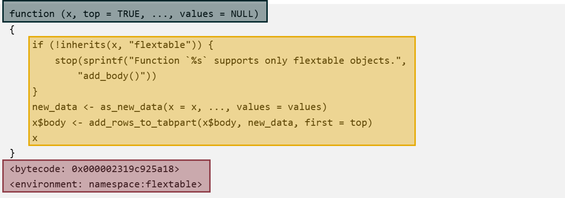
#load the required library for the functionlibrary(flextable)#run a function without the brackets to see what it is doingadd_body
function (x, top = TRUE, ..., values = NULL)
{
    if (!inherits(x, "flextable")) {
        stop(sprintf("Function `%s` supports only flextable objects.",
            "add_body()"))
    }
    new_data <- as_new_data(x = x, ..., values = values)
    x$body <- add_rows_to_tabpart(x$body, new_data, first = top)
    x
}
<bytecode: 0x0000021c4c78ff40>
<environment: namespace:flextable>
You would receive an output that looks like this: (minus the highlighting of course).
Look closely at the orange section and you will see that it is actually R code! Look even closer and you will see that it is running its own functions!
Here, fixed that meme for you:
Note
A small side note, the code in a function is not always R code, but that doesn’t really matter for us.
So whats the take away here?
Takeaway 1: You are already using functions in your code every day.
Takeaway 2: Its all just code, and if you are reading this you probably already code, and if you already code you can write your own functions no sweat!
Jokes aside, if it is all just code, why have functions? Generally speaking, functions are written because the thing they are doing gets done a whole lot. For example, I have to take the mean of a bunch of numbers in my job more times that I can count, and if I had to write out the inner workings of the mean function every time, I’d pull my hair out more times that I can count. The second reason functions are written can be called “abstraction”, essentially if a function has been well written then you don’t actually need to understand the code inside to be able to use it. In this way, I can run incredibly complicated statistical tests, or create my own website, or make interactive maps, without actually know the code to do these things - I just know how to use the functions that do these things.
Functions usually fill a specific niche, they do one thing really well, and nothing else. This also means that they are relatively simple, and if you felt like it you might even be able to dissect the function like we did above to see exactly how it works. (Although it is also perfectly fine to never worry about looking inside, don’t stress). In some cases you will encounter massive over complicated functions that do lots of seemingly unconnected things, but that is rarely true.
Functions that work well together, such as a whole heap of functions that work on tables, get bundled up together into “packages”. These is where the idea of “packages” comes from in R - you are just downloading a whole bunch of functions, which is just a whole bunch of code.
3 Making Your Own Functions
Okay its time to start talking about making your own functions. As we have covered, functions (particularly the ones you are going to write) are just R code. But obviously there is a little bit more to it than that. Lets look at the inside of a function again:
Overall, a function can be denoted as follows: your_function_name <- function(inputs){code} As we have covered, the orange part is the R code, that is the bit of code that gets executed when you use a function, and it goes inside the curly brackets. The dark green section at the top is the inputs section, where you tell the function what inputs to take, and what inputs are required. Inputs can also be called arguments. The red section at the bottom, for our purposes we can ignore that, it is metadata about the function and where it comes from.
The function as denoted above, then needs to be assigned to an object using the <- symbol. This makes the function like any other object in R where we can call it up later from our global environment. Lets make our first function to understand this better.
Code
#create a custom functioncustom_function_1 <-function(x){print(x)}#run our custom functioncustom_function_1(c(1,2,3))
[1] 1 2 3
Not the most thrilling demonstration I’ll admit that, but this is a really good demonstration of the connection between input and function - which is the next essential thing to understand about creating your own functions. When we look at this code we see “x” appear twice in the creation of the function, and then it is not used when we run the function. “x” is just a placeholder, much like over in my for loops blog, “x” can be anything! These two code chunks will execute and return the exact same result:
Code
#create a custom functioncustom_function_1 <-function(x){print(x)}#run our custom functioncustom_function_1(c(1,2,3))
Code
#create a custom functioncustom_function_1 <-function(SuperCoolPlaceholder){print(SuperCoolPlaceholder)}#run our custom functioncustom_function_1(c(1,2,3))
“x” is used to tell the function where the input goes. This is important because there can be more than one input in our function:
You can see here that “x” is 1, and “y” is 2, in truth the function can actually be used like this:
Code
custom_function_2(x =1, y =2)
[1] 1 2
And if you do write the code like that, then the order doesn’t matter:
Code
custom_function_2(y =2, x =1)
[1] 1 2
3.1 An Example of A Useful Custom Function
Anyway, lets actually create our own (useful) function. When I first understood how to create a function I was super excited to get started, but I quickly realized that I didn’t actually have a good reason to write a function. I find this is the case with a lot of intermediate coders, you might know the theory, but then finding places to implement it presents a whole new challenge. So lets refresh and hopefully come up with some good ideas:
Functions are bits of code that are used lots - is there anything code you have written that you have used more than once?
Functions usually do one thing really well - your first function doesn’t have to change the world!
There are thousands of functions already out there - the “best” problems probably already have functions written for them, focus on problems specific to your niche of work to find gaps.
Using these points, here are some ideas relevant to me (I encourage you to think of your own):
A function that cleans tables how I specifically like them to look (see here).
A function that run specific statistical calculates I use for my scientific reports.
A function that calculates landuse change by class (check out my long-form projects to read about this one).
A function that calculates important summary statistics about fish observations.
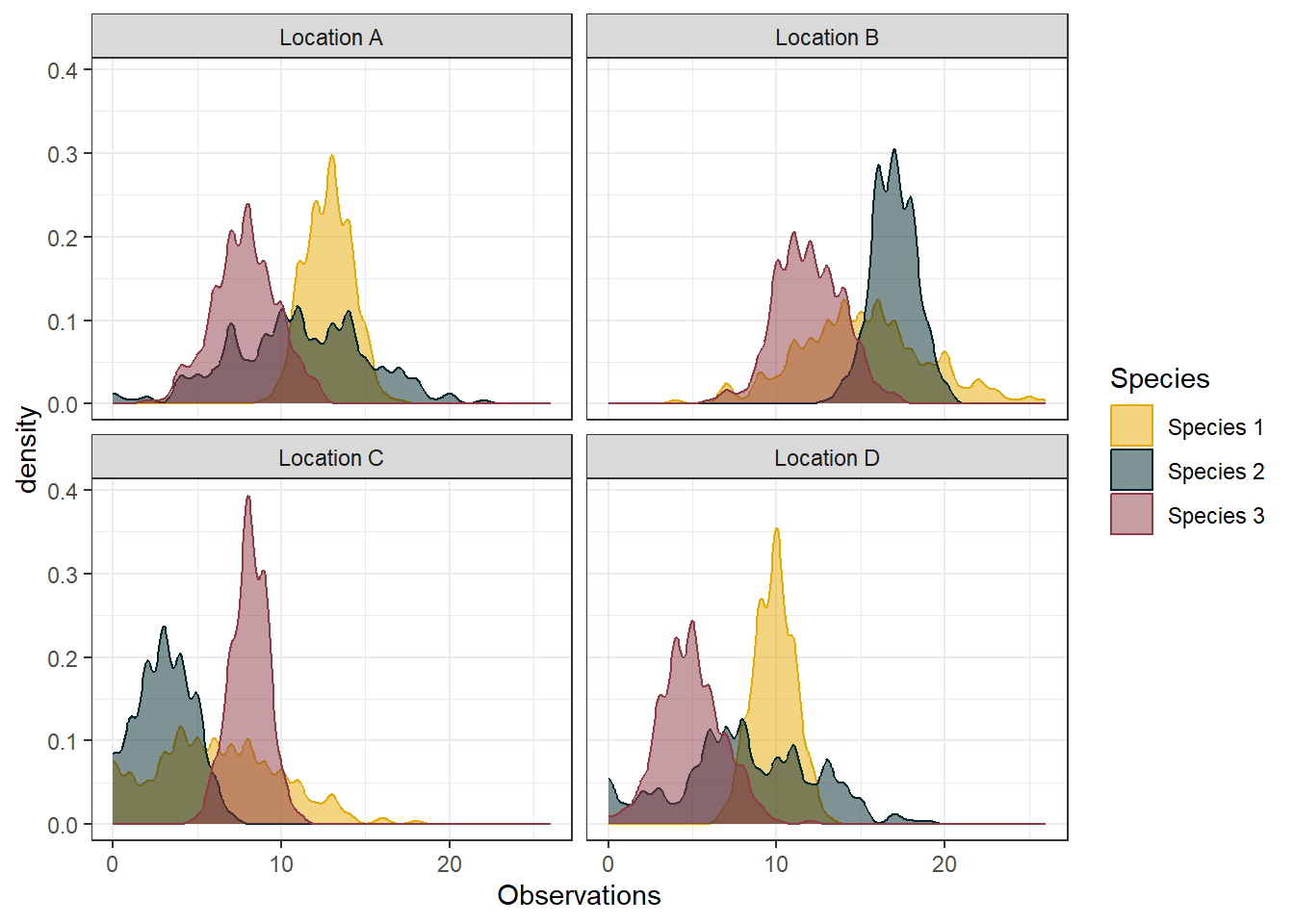
For demonstration purposes, lets learn together how to create that fourth function; calculating summary stats for fish observation data. First, here is some example data that I made up. It has observation counts for three different fish species across four different locations:
Code
#read in the example datasetfish_obs_df <-read.csv("fish_obs_df.csv")#view the dataframecond_form_tables(head(fish_obs_df, 10))
Location
Species
Observations
Location D
Species 2
0
Location B
Species 2
17
Location A
Species 3
9
Location A
Species 2
13
Location D
Species 1
9
Location C
Species 2
4
Location D
Species 2
15
Location C
Species 3
8
Location B
Species 3
10
Location A
Species 2
9
Code
#plot the dataggplot(fish_obs_df) +geom_density(aes(x=Observations, color = Species, fill = Species), bw =0.4, alpha =0.5) +scale_fill_manual(values =c("#e6aa04", "#00252A", "#8E3B46")) +scale_colour_manual(values =c("#e6aa04", "#00252A", "#8E3B46")) +theme_bw() +facet_wrap(~Location)
The data looks fairly standard. Normally, we probably then proceed to calculate some basic stats like the mean, median, min, max, etc. So lets do that:
Code
#generic summary statssummary_table <- fish_obs_df |>group_by(Location, Species) |>summarise(Mean =round(mean(Observations),2),Median =median(Observations),Min =min(Observations),Max =max(Observations),Range = Max - Min) |>ungroup()#print the tablecond_form_tables(summary_table)
Location
Species
Mean
Median
Min
Max
Range
Location A
Species 1
12.8
13
9
17
8
Location A
Species 2
11
11
0
22
22
Location A
Species 3
7.82
8
2
12
10
Location B
Species 1
15.1
15
4
26
22
Location B
Species 2
17
17
13
20
7
Location B
Species 3
11.9
12
6
17
11
Location C
Species 1
6.11
6
0
18
18
Location C
Species 2
3.03
3
0
7
7
Location C
Species 3
8.08
8
5
11
6
Location D
Species 1
9.84
10
7
13
6
Location D
Species 2
8.09
8
0
19
19
Location D
Species 3
4.94
5
0
12
12
Cool, and for fun, lets also say that we are interested to know how many times the observation count of the species was above 10 at each site:
Code
#number of observations above nsummary_table_2 <- fish_obs_df |>filter(Observations >10) |>group_by(Location, Species) |>summarise(CountAbove10 =n()) |>ungroup()#add the count to the main tablesummary_table <-left_join(summary_table, summary_table_2)#print the tablecond_form_tables(summary_table)
Location
Species
Mean
Median
Min
Max
Range
CountAbove10
Location A
Species 1
12.8
13
9
17
8
238
Location A
Species 2
11
11
0
22
22
136
Location A
Species 3
7.82
8
2
12
10
20
Location B
Species 1
15.1
15
4
26
22
225
Location B
Species 2
17
17
13
20
7
256
Location B
Species 3
11.9
12
6
17
11
192
Location C
Species 1
6.11
6
0
18
18
34
Location C
Species 2
3.03
3
0
7
7
Location C
Species 3
8.08
8
5
11
6
3
Location D
Species 1
9.84
10
7
13
6
69
Location D
Species 2
8.09
8
0
19
19
73
Location D
Species 3
4.94
5
0
12
12
1
Now, for the purposes of this learning experience, lets say that this initial analysis above is something that I will need to do every time I load a dataset, and is therefore a perfect time to write a function to do the analysis for me. So do I go from the code I have written to a function? Like this:
Identify the code to go in the function (we’ve done this).
Put the code inside the function wrapper my_custom_function <- function(input){right here!}:
Code
my_custom_function <-function(inputs){#generic summary stats summary_table <- fish_obs_df |>group_by(Location, Species) |>summarise(Mean =round(mean(Observations),2),Median =median(Observations),Min =min(Observations),Max =max(Observations),Range = Max - Min) |>ungroup()#number of observations above n summary_table_2 <- fish_obs_df |>filter(Observations >10) |>group_by(Location, Species) |>summarise(CountAbove10 =n()) |>ungroup()#add the count to the main table summary_table <-left_join(summary_table, summary_table_2)}
Identify the inputs required for the code to run:
Code
my_custom_function <-function(inputs){#generic summary stats summary_table <- fish_obs_df |>#the fish_obs_df dataset is an input, we need to tell the function what dataset to usegroup_by(Location, Species) |>#the Location and Species columns are inputs, we need to tell the function what columns to group bysummarise(Mean =round(mean(Observations),2), #the Observation column is an input, we need to tell the function what columns calculate onMedian =median(Observations),Min =min(Observations),Max =max(Observations),Range = Max - Min) |>ungroup()#number of observations above n summary_table_2 <- fish_obs_df |>filter(Observations >10) |>#the value 10 is an input, we need to tell the function what cut off value to usegroup_by(Location, Species) |>summarise(CountAbove10 =n()) |>ungroup()#add the count to the main table summary_table <-left_join(summary_table, summary_table_2)}
Looks like we have five different inputs, next we give each of those inputs their own placeholder:
Code
my_custom_function <-function(x,y,z,a,b){#generic summary stats summary_table <- x |>#the fish_obs_df dataset is now "x"group_by({{y}}, {{z}}) |>#the Location and Species columns are now "y" and "z" we need to use curly-curly brackets for column names provided externallysummarise(Mean =round(mean({{a}}),2), #the Observation column is now "a"Median =median({{a}}),Min =min({{a}}),Max =max({{a}}),Range = Max - Min) |>ungroup()#number of observations above n summary_table_2 <- x |>filter({{a}} > {{b}}) |>#the value is now "b"group_by({{y}}, {{z}}) |>summarise(CountAbove10 =n()) |>ungroup()#add the count to the main table summary_table <-left_join(summary_table, summary_table_2)}
Specify the output of the function:
Code
my_custom_function <-function(x,y,z,a,b){#generic summary stats summary_table <- x |>group_by({{y}}, {{z}}) |>summarise(Mean =round(mean({{a}}),2), Median =median({{a}}),Min =min({{a}}),Max =max({{a}}),Range = Max - Min) |>ungroup()#number of observations above n summary_table_2 <- x |>filter({{a}} > {{b}}) |>group_by({{y}}, {{z}}) |>summarise(CountAbove10 =n()) |>ungroup()#add the count to the main table summary_table <-left_join(summary_table, summary_table_2)#what should be returned?return(summary_table)}
Run the function:
Code
my_custom_function <-function(x,y,z,a,b){#generic summary stats summary_table <- x |>group_by({{y}}, {{z}}) |>summarise(Mean =round(mean({{a}}),2), Median =median({{a}}),Min =min({{a}}),Max =max({{a}}),Range = Max - Min) |>ungroup()#number of observations above n summary_table_2 <- x |>filter({{a}} > {{b}}) |>#the value is now "b"group_by({{y}}, {{z}}) |>summarise(CountAbove10 =n()) |>ungroup()#add the count to the main table summary_table <-left_join(summary_table, summary_table_2)#what should be returned?return(summary_table)}
now, if we run the code, the function will appear in your global environment on the right. Congratulations, you just made a function. Lets see if it works:
Ok, spoiler, we are not actually done yet. First of all, lets make those place holders more helpful:
Code
my_custom_function <-function(df, group_col_1, group_col_2, value, cut_off_value){#generic summary stats summary_table <- df |>group_by({{group_col_1}}, {{group_col_2}}) |>summarise(Mean =round(mean({{value}}),2), Median =median({{value}}),Min =min({{value}}),Max =max({{value}}),Range = Max - Min) |>ungroup()#number of observations above n summary_table_2 <- df |>filter({{value}} > {{cut_off_value}}) |>group_by({{group_col_1}}, {{group_col_2}}) |>summarise(CountAbove10 =n()) |>ungroup()#add the count to the main table summary_table <-left_join(summary_table, summary_table_2)#what should be returned?return(summary_table)}
Secondly, lets make the column name for the cut off value adaptive to the actual cut off value:
Code
my_custom_function <-function(df, group_col_1, group_col_2, value, cut_off_value){#generic summary stats summary_table <- df |>group_by({{group_col_1}}, {{group_col_2}}) |>summarise(Mean =round(mean({{value}}),2), Median =median({{value}}),Min =min({{value}}),Max =max({{value}}),Range = Max - Min) |>ungroup()#number of observations above n summary_table_2 <- df |>filter({{value}} > {{cut_off_value}}) |>group_by({{group_col_1}}, {{group_col_2}}) |>summarise(!!sym(glue("CountAbove{cut_off_value}")) :=n()) |>#we have to use !!sym() when the name is not named col. We also use ":=" in place of the normal equalsungroup()#add the count to the main table summary_table <-left_join(summary_table, summary_table_2)#what should be returned?return(summary_table)}
Third, lets identify what kind of dependencies this function has, i.e., what kind of functions does it rely on and what packages would we have to load for it to work:
Code
my_custom_function <-function(df, group_col_1, group_col_2, value, cut_off_value){#load the required packageslibrary(dplyr)library(glue)#generic summary stats summary_table <- df |>group_by({{group_col_1}}, {{group_col_2}}) |>summarise(Mean =round(mean({{value}}),2), Median =median({{value}}),Min =min({{value}}),Max =max({{value}}),Range = Max - Min) |>ungroup()#number of observations above n summary_table_2 <- df |>filter({{value}} > {{cut_off_value}}) |>#the value is now "b"group_by({{group_col_1}}, {{group_col_2}}) |>summarise(!!sym(glue("CountAbove{cut_off_value}")) :=n()) |>ungroup()#add the count to the main table summary_table <-left_join(summary_table, summary_table_2)#what should be returned?return(summary_table)}
Forth, what if the packages haven’t been installed? Lets add a check and warning for this:
Code
my_custom_function <-function(df, group_col_1, group_col_2, value, cut_off_value){#set a vector of names of packages we need pkg <-c("dplyr", "glue")# Loop through each packagefor (p in pkg) {if (!requireNamespace(p, quietly =TRUE)) {warning(sprintf("The package '%s' is not installed. Please install it with install.packages('%s')", p, p)) } else {library(p, character.only =TRUE) } }#generic summary stats summary_table <- df |>group_by({{group_col_1}}, {{group_col_2}}) |>summarise(Mean =round(mean({{value}}),2), Median =median({{value}}),Min =min({{value}}),Max =max({{value}}),Range = Max - Min) |>ungroup()#number of observations above n summary_table_2 <- df |>filter({{value}} > {{cut_off_value}}) |>#the value is now "b"group_by({{group_col_1}}, {{group_col_2}}) |>summarise(!!sym(glue("CountAbove{cut_off_value}")) :=n()) |>ungroup()#add the count to the main table summary_table <-left_join(summary_table, summary_table_2)#what should be returned?return(summary_table)}
Now this is starting to look like a real function! Lets do some testing to make sure those adjustments worked fine:
Looking good to me. What we have now is our very own custom function that:
takes a dataframe, two grouping columns, a value column, and a cut-off/objective value
and returns a summary dataframe as well as the number of observations that were above the cut-off
However, there is still one glaring gap that I find alot of tutorials skip over… this code is still in the same script! All we have really done is make it longer and slightly abstracted so far!
The final stage of creating our custom function is saving and tucking away the function somewhere else so we can then refer to it later as we need. Doing this is not to hard:
Open a new R script. Not a .qmd file, or a markdown file, a pure R script.
Copy and paste the custom function into the new R script.
Save this script somewhere relevant, I like to create a folder in my work space called “functions”.
Done. To access the function that we just put inside the script we then write the following code:
Code
source("path_to_script/script_name.R")
This will load the function into your global environment ready for use.
4 Additional Resources
Ok so I will admit, that is a lot. No matter which way you slice it, the first time you start getting into functions there is going to be a lot to learn. Its an continual process, and one of the best things you can do is have a good amount of material to refer back to anytime you get stuck. One of my favourite resources for learning everything there is to know about functions would be the R for Data Science book by Hadley Wickham. Second to this, for quick fixes you can of course use chatGPT. ChatGPT is quite good at puzzling out semantic and grammatical errors - of which functions can have plenty.
5 Caveats
While functions can be powerful, they can also be dangerous - driving the unwary coder insane while trying to debug their own poorly written work (guilty). It is often tossed around that “any code repeated more than once should be put in a function or loop”. Personally I think this is an over simplification that can lead to significant time losses in the wrong situation. In some cases, sure you should probably put that repeated code in a function, but other times the repeat is so simple that the added complexity of a function is unnecessary. Equally, there are also instances in which the “repeated” code is a convoluted web of moving parts that creating a function to adequately encompass it all is a nightmare. All this is to say, don’t get drunk on your new found power and try to put everything you do into a function - you’ll quickly burn out and maybe even be turned away from functions for ever. Be pragmatic about your implementation, and enjoy it.
Thanks For Reading!
If you like the content, please consider donating to let me know. Also please stick around and have a read of several of my other posts. You'll find work on everything from simple data management and organisation skills, all the way to writing custom functions, tackling complex environmental problems, and my journey when learning new environmental data analyst skills.